'Code'에 해당되는 글 161건
-
!['[Python] LinearRegression(수치예측)' 포스트 대표 이미지](https://img1.daumcdn.net/thumb/R750x0/?scode=mtistory2&fname=https%3A%2F%2Fblog.kakaocdn.net%2Fdna%2F94VOO%2FbtqxPTHHDn2%2FAAAAAAAAAAAAAAAAAAAAAFCbaThqIxP-QE7Fnhs-tv2uIqoFcAtu3nzv4PcEFV-R%2Fimg.png%3Fcredential%3DyqXZFxpELC7KVnFOS48ylbz2pIh7yKj8%26expires%3D1772290799%26allow_ip%3D%26allow_referer%3D%26signature%3DIXugsG%252BtOdUpSrbpm965LB%252BdVbI%253D) [Python] LinearRegression(수치예측)2019.08.28
[Python] LinearRegression(수치예측)2019.08.28 -
!['[Python] Gradient Boosting' 포스트 대표 이미지](https://img1.daumcdn.net/thumb/R750x0/?scode=mtistory2&fname=https%3A%2F%2Fblog.kakaocdn.net%2Fdna%2F9mDmi%2FbtqxMsdE89k%2FAAAAAAAAAAAAAAAAAAAAAHhPR4QMYE_Yy8XcAzWkEfcaN7REYq0c6hmsMvbDUho3%2Fimg.png%3Fcredential%3DyqXZFxpELC7KVnFOS48ylbz2pIh7yKj8%26expires%3D1772290799%26allow_ip%3D%26allow_referer%3D%26signature%3Dd1pm3Nl4CYu%252Bvw0xu9dYBOLxGD0%253D) [Python] Gradient Boosting2019.08.28
[Python] Gradient Boosting2019.08.28 -
!['[Python] RandomForest 예제' 포스트 대표 이미지](https://img1.daumcdn.net/thumb/R750x0/?scode=mtistory2&fname=https%3A%2F%2Fblog.kakaocdn.net%2Fdna%2FbIl3sU%2FbtqxKrzhDIg%2FAAAAAAAAAAAAAAAAAAAAAEIsXw5fAlQZRfhV-vX_XeBI7aqjdORbRo2ZJzPD8ZT1%2Fimg.png%3Fcredential%3DyqXZFxpELC7KVnFOS48ylbz2pIh7yKj8%26expires%3D1772290799%26allow_ip%3D%26allow_referer%3D%26signature%3DzzzEvZ7xAtnclOBn2HY9LI74iM4%253D) [Python] RandomForest 예제2019.08.27
[Python] RandomForest 예제2019.08.27 -
!['[Python] RandomForest' 포스트 대표 이미지](https://img1.daumcdn.net/thumb/R750x0/?scode=mtistory2&fname=https%3A%2F%2Fblog.kakaocdn.net%2Fdna%2FOsAjl%2FbtqxKq1osXO%2FAAAAAAAAAAAAAAAAAAAAAG62p_Mlg_HcsEWl-3TXWgkJKXCgY8OUne40IYBgipbk%2Fimg.png%3Fcredential%3DyqXZFxpELC7KVnFOS48ylbz2pIh7yKj8%26expires%3D1772290799%26allow_ip%3D%26allow_referer%3D%26signature%3D6M9W%252FW7pgHSrOo0TePjcXK5jbOU%253D) [Python] RandomForest2019.08.27
[Python] RandomForest2019.08.27 -
!['[Python] DecisionTree' 포스트 대표 이미지](https://img1.daumcdn.net/thumb/R750x0/?scode=mtistory2&fname=https%3A%2F%2Fblog.kakaocdn.net%2Fdna%2FWjbBm%2FbtqxKBBD8Za%2FAAAAAAAAAAAAAAAAAAAAADdePnYMWnqQdZM_WcL9KTXMfn_IedTX1nRbfIZABjIJ%2Fimg.png%3Fcredential%3DyqXZFxpELC7KVnFOS48ylbz2pIh7yKj8%26expires%3D1772290799%26allow_ip%3D%26allow_referer%3D%26signature%3DZ0813MVNmheuHlbaMLVcxojXg50%253D) [Python] DecisionTree2019.08.27
[Python] DecisionTree2019.08.27 -
!['[Python] k-nearest neighbor 예제' 포스트 대표 이미지](https://img1.daumcdn.net/thumb/R750x0/?scode=mtistory2&fname=https%3A%2F%2Fblog.kakaocdn.net%2Fdna%2F1XJ1W%2FbtqxQo3C3oY%2FAAAAAAAAAAAAAAAAAAAAABSqvtZ6Y8Z4KEh0C557lfhUV4zEhRhgA-HsulKmlIWa%2Fimg.png%3Fcredential%3DyqXZFxpELC7KVnFOS48ylbz2pIh7yKj8%26expires%3D1772290799%26allow_ip%3D%26allow_referer%3D%26signature%3DRRtDIEWseePsfQ84y%252FDzI9wK8VE%253D) [Python] k-nearest neighbor 예제2019.08.26
[Python] k-nearest neighbor 예제2019.08.26 -
[Python]k-nearest neighbor2019.08.26
-
텍스트 분석_BOW2019.08.14
-
텍스트 분석_텍스트 전처리 22019.08.14
-
텍스트 분석_텍스트 전처리12019.08.13
[Python] LinearRegression(수치예측)
Linear Regression(수치예측) : 선형회귀분석
- 종속변수 y와 한 개 이상의 독립변수(설명변수) x와의 선형 상관 관계를 모델링 하는 회귀분석 기법
- 선형 회귀를 사용해 데이터에 적합한 예측 모형을 개발해 값 예측 가능
- 일반적으로 최소제곱법을 이용해 모델 세움( 손실 함수도 사용 가능)
- 단순 선형 회귀, 다중 선형 회귀
1. 단순 선형 회귀 - diabetes 데이터 이용
# 0. 라이브러리 불러오기
from sklearn.linear_model import LinearRegression
from sklearn import datasets
from sklearn.model_selection import train_test_split
import matplotlib.pyplot as plt
import numpy as np
import pandas as pd


# 1. diabetes dataset loading
diab = datasets.load_diabetes()


# 2. 네번째 feature 선택 -> 선형이기 때문에 하나의 x에 대해서만!
diab_X = diabetes.data[:,np.newaxis,3]  # 네번째 있는 칼럼을 수직방향으로 뽑아줌


# 3. 데이터 추출 확인
diab_X[0]


# 4. split data
diab_X_train = diab_X[:-20]
diab_X_test = diab_X[-20:]

diab_y_train = diab.target[:-20]
diab_y_test = diab.target[-20:]


# 5 모델 객체 생성 및 fitting
lr = LinearRegression()
lr.fit(diab_X_train, diab_y_train)


# 6 prediction
diab_pred = lr.predict(diab_X_test)


# 7 훈련 결과 확인
print("훈련 세트 점수 : {:.3f}".format(lr.score(diab_X_train,diab_y_train)))
print("테스트 세트 점수 : {:.3f}".format(lr.score(diab_X_test,diab_y_test)))
# 결과 : 훈련 세트 점수 : 0.192  테스트 세트 점수 : 0.160

# 그래프
plt.scatter(diab_X_test, diab_y_test, color='black')
plt.plot(diab_X_test, diab_pred, color="blue", linewidth=3)

plt.show()
단순 선형 회귀를 통한 결과를 그래프로 보면 위와 같다.
2. 다중 선형 회귀 - boston 데이터 이용
# 0. 라이브러리 추가
from sklearn.datasets import load_boston
boston = load_boston()

# 1. 데이터 분류
X = boston.data
y = boston.target

X_train, X_test, y_train, y_test = train_test_split(X,y,test_size=0.3,random_state = 12)

# 2. 모델링
lr = LinearRegression().fit(X_train, y_train)

# 3. 결과 확인
print("훈련 세트 점수 : {:.3f}".format(lr.score(X_train,y_train)))
print("테스트 세트 점수 : {:.3f}".format(lr.score(X_test,y_test)))
# 훈련 세트 점수 : 0.748 테스트 세트 점수 : 0.709
다중 회귀 방식이기 때문에 선형 회귀와 다르게 그래프를 그리지 못해 생략했습니다.
'Code > 머신러닝 in Python' 카테고리의 다른 글
| [Python] LinearRegression(수치예측) - Lasso (0) | 2019.08.28 |
|---|---|
| [Python] LinearRegression(수치예측) - Ridge (0) | 2019.08.28 |
| [Python] Gradient Boosting (0) | 2019.08.28 |
| [Python] RandomForest 예제 (0) | 2019.08.27 |
| [Python] RandomForest (0) | 2019.08.27 |
[Python] Gradient Boosting
Gradient Boosting
**특징
- 여러개의 결정트리를 묶어 강력한 모델을 만듦
- RF와 달리 이전 트리의 오차를 보완하는 방식으로 순차적으로 트리 생성 -> 무작위성이 없음
- 강력한 사전가지치기 사용
- 보통 5가지 이하의 얕은 트리를 사용 -> 적은 메모리
- 얕은 트리(weak learner로 통칭)를 많이 연결, 각 트리는 데이터의 일부에 대해서만 예측을 수행 -> 트리를 많이 추가할 수록 성능이 좋아짐
**주요 매개변수
- 사전가지치기, 트리의 개수 외에
- learning rate: 이전 트리의 오차를 얼마나 강하게 보장할 것인지를 제어 -> 학습률이 크면 보정을 강하게 하므로 모델의 복잡도 증가
- iris 데이터를 이용한 Gradient Boosting 작업 순서
# 필요한 라이브러리 추가
from sklearn.ensemble import GradientBoostingClassifier
from sklearn.model_selection import train_test_split
from sklearn import datasets


# 1 데이터 로딩
iris = datasets.load_iris()

# 2 데이터 분할
X = iris.data
y = iris.target

X_train, X_test, y_train, y_test= train_test_split(X,y,test_size=0.3,random_state = 10)

# 3 모델 객체 생성
gtb = GradientBoostingClassifier()  # default 값 max_depth = 3

# 4 fitting model
gtb.fit(X_train, y_train)

# 5 훈련 데이터
print("훈련 세트 점수 : {:.3f}".format(gtb.score(X_train,y_train)))
print( "테스트 세트 점수 : {:.3f}".format(gtb.score(X_test,y_test)))

위와 같이 default로 사용할 경우 이미지와 같은 GradientBoostingClassifier가 만들어집니다.
훈련 세트 점수 : 1.000 테스트 세트 점수 : 0.978
적합한 max_depth를 찾고 n_en_estimators 를 찾는 과정을 예제를 통해 학습해보겠습니다.
breast_cancer 데이터 이용해 분석하기
# 1. 데이터 불러오기
from sklearn.datasets import load_breast_cancer
breast = load_breast_cancer()


# 2. 데이터 분류
Xb = breast.data
yb = breast.target
Xb_train, Xb_test, yb_train, yb_test = train_test_split(Xb, yb, test_size=0.3, random_state = 43)


# 3. modelling

## 3.1 max_depth = 1
gtb1 = GradientBoostingClassifier(max_depth=1).fit(Xb_train, yb_train)
print("훈련 세트 점수 : {:.3f}".format(gtb1.score(Xb_train,yb_train)))
print( "테스트 세트 점수 : {:.3f}".format(gtb1.score(Xb_test,yb_test)))
# 결과 : 훈련 세트 점수 : 0.990  테스트 세트 점수 : 0.977


## 3.2 max_depth = 2
gtb2 = GradientBoostingClassifier(max_depth=2).fit(Xb_train, yb_train)
print("훈련 세트 점수 : {:.3f}".format(gtb2.score(Xb_train,yb_train)))
print( "테스트 세트 점수 : {:.3f}".format(gtb2.score(Xb_test,yb_test)))
# 결과 : 훈련 세트 점수 : 1.000 테스트 세트 점수 : 0.977


## 3.3 max_depth = 3
gtb3 = GradientBoostingClassifier(max_depth=3).fit(Xb_train, yb_train)
print("훈련 세트 점수 : {:.3f}".format(gtb3.score(Xb_train,yb_train)))
print( "테스트 세트 점수 : {:.3f}".format(gtb3.score(Xb_test,yb_test)))
# 결과 : 훈련 세트 점수 : 1.000 테스트 세트 점수 : 0.977

# 위의 결과를 봤을 때, max_depth = 2일 때 적합하다고 예상할 수 있습니다.


# 4. 모델링 반복(max_depth = 2를 이용하여)
train_acc, test_acc = [],[]
n_estimators = range(5,201,5)

for n_estimator in n_estimators:
    # 모델 생성
    gtb3_depth_n = GradientBoostingClassifier(n_estimators=n_estimator, random_state=n_estimator, max_depth=2)

    gtb3_depth_n.fit(Xb_train, yb_train)

    train_acc.append(gtb3_depth_n.score(Xb_train, yb_train))
    test_acc.append(gtb3_depth_n.score(Xb_test, yb_test))

# 5. estimator 변화에 따른 결과 그래프로 확인
import matplotlib.pyplot as plt

plt.figure(figsize = (20,10))
plt.plot(n_estimators, train_acc, label="train",marker='o')
plt.plot(n_estimators, test_acc, label="test",marker='o')
plt.ylabel('accuracy')
plt.xlabel('number of n_estimators')
plt.legend(fontsize=15)


# 6. 최종 모델 확인
gtb3_depth_n = GradientBoostingClassifier(n_estimators=155, random_state=155, max_depth=2, learning_rate=0.1)
gtb3_depth_n.fit(Xb_train, yb_train)

# 훈련 정확도 출력
print("훈련 세트 점수 : {:.3f}".format(gtb3_depth_n.score(Xb_train,yb_train)))
print( "테스트 세트 점수 : {:.3f}".format(gtb3_depth_n.score(Xb_test,yb_test)))

# learning_rate를 높이면 보정을 강하게 하기 때문에 복잡한 모델을 만듭니다.(default = 0.1)
# n_estimator 값을 키우면 ensemble에 트리가 더 많이 추가되어 모델의 복잡도가 커지고 train 세트를 더 정확하게 fitting합니다.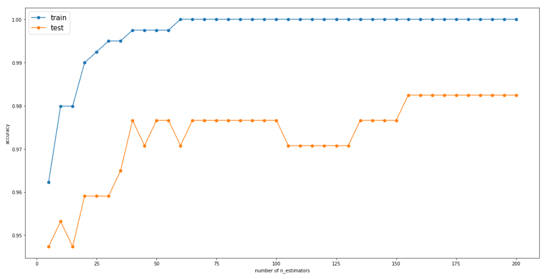
훈련 세트 점수 : 1.000 테스트 세트 점수 : 0.982
위의 그래프를 확인하면 n_esimators가 155일 때가 가장 높은 test 점수를 가지기 때문에 155로 모델에 적용시킨 후 최종 결과를 뽑아냈습니다.
간단하게 gradient boosting 에 대해 공부해보았습니다.
궁금한 사항, 부족한 사항은 댓글에 담겨주세요!
'Code > 머신러닝 in Python' 카테고리의 다른 글
| [Python] LinearRegression(수치예측) - Ridge (0) | 2019.08.28 |
|---|---|
| [Python] LinearRegression(수치예측) (0) | 2019.08.28 |
| [Python] RandomForest 예제 (0) | 2019.08.27 |
| [Python] RandomForest (0) | 2019.08.27 |
| [Python] DecisionTree (0) | 2019.08.27 |
[Python] RandomForest 예제
- breast_cancer 데이터를 이용하여 적합한 randomforest의 트리 개수와, 특정값을 구해보자
# 1 데이터 호출
from sklearn.datasets import load_breast_cancer
breast_cancer_dataset = load_breast_cancer()

# 1-1 데이터 분류
X_train,X_test,y_train,y_test = train_test_split(X,y, test_size = 0.3, random_state = 10)

# 2 n_estimators
depths=range(5,201,5)
forest_train,forest_test = [],[]

for i in depths:
    forest = RandomForestClassifier(n_estimators=i, random_state=i)
    forest.fit(X_train,y_train)

    forest_train.append(forest.score(X_train,y_train))
    forest_test.append(forest.score(X_test,y_test))

plt.plot(depths,forest_train,label='훈련 정확도',marker='o')
plt.plot(depths,forest_test,label='테스트 정확도',marker='o')
plt.ylabel('accuracy')
plt.xlabel('number of n_estimators')
plt.legend()
2. n_n_estimators 는 randomforest에서 의사결정나무의 개수를 정해준다고 했습니다.
그럼 적합한 나무의 개수가 무엇인지 확인하기 위해 range를 통해 다양한 숫자를 넣어 그래프로 train,test의 정확도를 확인해보았습니다. (random_state도 같이 증가시켜 확인해보았습니다)
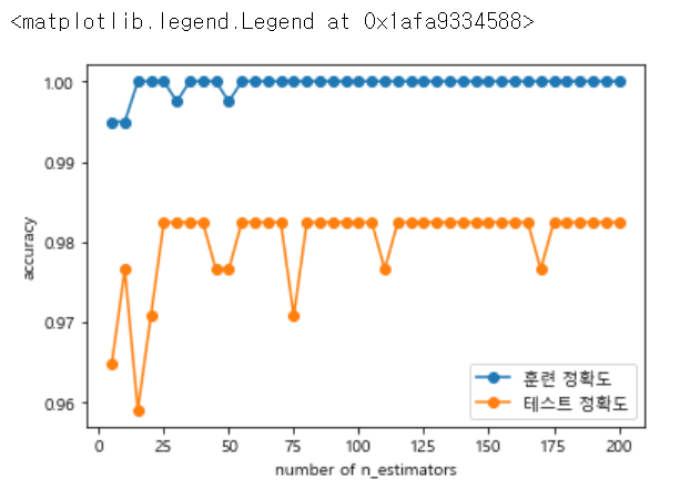
위의 그래프를 보면 test 정확도가 25일때 가장 최대이며, 더 이상 높아지지 않다는 것을 추정하면 n_estimators = 25로 지정할 수 있습니다.
# 3 max_features
depths=range(1,31)

tree_train,tree_test = [],[]

for i in depths:
    forest = RandomForestClassifier(n_estimators=25, random_state=25, max_features=i)
    forest.fit(X_train,y_train)

    tree_train.append(forest.score(X_train,y_train))
    tree_test.append(forest.score(X_test,y_test))

plt.plot(depths,tree_train,label='훈련 정확도',marker='o')
plt.plot(depths,tree_test,label='테스트 정확도',marker='o')
plt.ylabel('accuracy')
plt.xlabel('number of max_features')
plt.legend()
3 max_features 에서는 적합한 features의 수를 구하기 위한 작업입니다.
위에서 높게 나온 n_estimators와 random_state를 25로 지정해높고 1~ 31까지 반복문을 돌려줍니다.
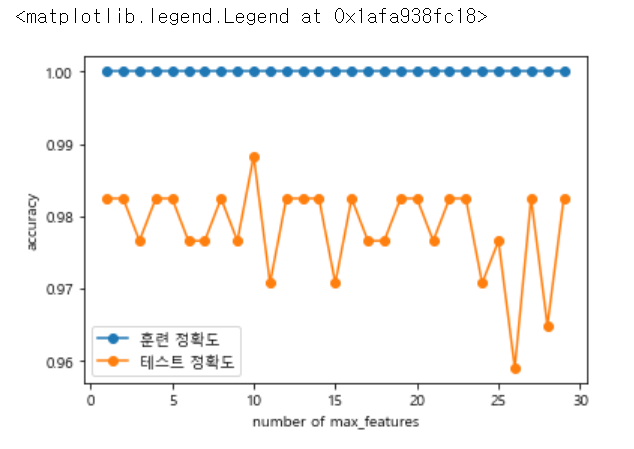
위 그래프에서 test가 제일 높을 때 max_features의 값은 10인 것을 확인할 수 있습니다.
# 최종 확인
forest = RandomForestClassifier(n_estimators=25, random_state=25, max_features=10)
forest.fit(X_train,y_train)

print("train accuracy {:.2f}".format(forest.score(X_train,y_train)))
print("test accuracy {:.2f}".format(forest.score(X_test, y_test)))
마지막 최종확인으로 가장 적합한 값을 넣어서 최종 train, test 정확도를 확인해보았습니다.
train accuracy 1.00
test accuracy 0.99
이상으로 randomforest 모델을 이용하는 것을 공부했습니다.
'Code > 머신러닝 in Python' 카테고리의 다른 글
| [Python] LinearRegression(수치예측) (0) | 2019.08.28 |
|---|---|
| [Python] Gradient Boosting (0) | 2019.08.28 |
| [Python] RandomForest (0) | 2019.08.27 |
| [Python] DecisionTree (0) | 2019.08.27 |
| [Python] k-nearest neighbor 예제 (0) | 2019.08.26 |
[Python] RandomForest
What is Random Forest
- 여러개의 Decision Tree를 사용하는 앙상블 분류모형의 일종
- 앙상블의 사전적 의미 : 1.음악 ( 2인 이상에 의한 가창이나 연주) 2.음악 ( 주로 실내악을 연주하는 소인원의 합주단*합창단)
- 앙상블 러닝이 생겨난 배경 : 실제 데이터는 상당히 복잡하고, 여러 다양한 컨셉을 포함한. 따라서, 하나의 모델로 제대로 설명해내는데 어려움이 있음
- 앙상블은 여러 다른 모델의 결과를 결합하여 사용함으로써, 일반적으로 하나의 모델을 사용한 것보다 분석 결과가 좋음
랜덤포레스트를 위해 파이썬에서 임의의 데이터 셋을 만들어 확인해보겠습니다.
from sklearn.ensemble import RandomForestClassifier
from sklearn import datasets
from sklearn.model_selection import train_test_split
import numpy as np
import matplotlib.pyplot as plt

# 1. toy 데이터 생성하기
X, y = datasets.make_moons(n_samples=100, noise=0.25, random_state=3)

# 1.1 데이터 확인
X.shape

plt.scatter(X[:,0],X[:,1],edgecolors='red',s=50,c=y)

# 1.2 데이터 분할
X_train,X_test,y_train,y_test = train_test_split(X,y, test_size = 0.2, random_state = 1234)

# 1.3 분할 데이터 확인
X_train.shape, y_train.shape

# 2. random forest 모델링을 위할 객체 생성
# n_estimators : 만들 의사결정나무 개수
forest = RandomForestClassifier(n_estimators=5, random_state=5)

# 3. 모델 적합
forest.fit(X_train, y_train)

# 4. 결과 확인
print("train accuracy {:.2f}".format(forest.score(X_train, y_train)))
print("test accuracy {:.2f}".format(forest.score(X_test, y_test)))

# 5 트리 확인
forest.estimators_

# 5-1 트리 일부 확인
export_graphviz(forest.estimators_[0], out_file = "rf{}.dot".format(0),
                rounded=True, proportion=False,
                filled=True, precision=2)
with open("rf{}.dot".format(0)) as f1:
    dot_graph1 = f1.read()
graphviz.Source(dot_graph1)

소스를 작동하면 다음과 같은 의사결정나무0 이 출력되게 됩니다!
랜덤포레스트가 어떤 의사결정나무로 구성되었는지 확인하고 싶으면
export_graphviz(forest.estimators_[0], out_file = "rf{}.dot".format(0),
                rounded=True, proportion=False,
                filled=True, precision=2)
with open("rf{}.dot".format(0)) as f1:
    dot_graph1 = f1.read()
graphviz.Source(dot_graph1)
여기서 0을 5까지 변경시켜보면서 확인할 수 있습니다.
'Code > 머신러닝 in Python' 카테고리의 다른 글
| [Python] Gradient Boosting (0) | 2019.08.28 |
|---|---|
| [Python] RandomForest 예제 (0) | 2019.08.27 |
| [Python] DecisionTree (0) | 2019.08.27 |
| [Python] k-nearest neighbor 예제 (0) | 2019.08.26 |
| [Python]k-nearest neighbor (0) | 2019.08.26 |
[Python] DecisionTree
DecisionTree : 의사결정나무
- 어떤 항목에 대한 관측값과 목표값을 연결시켜주는 예측모델
- 시각적이고 명시적인 방법으로 의사 결정 과정과 결정된 의사를 보여주는 데 사용
- 데이터 분할을 하기 위해, 가장 훌륭한 변수가 무엇인지 찾아야함
간단한 파이썬으로 iris 데이터를 의사결정나무로 에측해본 것입니다.
# Decision Tree

# 필요 모듈 import
from sklearn.tree import DecisionTreeClassifier
from sklearn.datasets import load_iris
from sklearn import tree
from sklearn.model_selection import train_test_split

# 사이킷런의 iris 데이터 불러오기
iris_dataset = load_iris()

# data split
X = iris_dataset.data
y = iris_dataset.target
X_train, X_test, y_train, y_test = train_test_split(X,y,test_size=0.3, random_state = 25)

# 객체 생성
# max_depth : 사용자 설정에 따라 tree의 레벨 조정 가능
clf = tree.DecisionTreeClassifier(max_depth=None, random_state=0)

# 모델링
clf.fit(X_train, y_train)

print("훈련 세트 점수 {:3f}".format(clf.score(X_train, y_train)))
print("테스트 세트 점수 {:3f}".format(clf.score(X_test, y_test)))
여기서 해당 모델에 대해 시각적으로 확인하고 싶으면
# 아나콘다에서 설치 필요
#conda install graphviz
#conda install python-graphviz


import os

# 환경변수 조정
os.environ['PATH']+=os.pathsep+'C:/Anaconda3/Library/bin/graphviz/'

# 모델 저장
export_graphviz(clf, out_file = "iris.dot",
               feature_names=cancer.feature_names,
               class_names=cancer.target_names,
               rounded=True, proportion=False,
               filled=True, precision=2)

# 파일로 불러오기
with open("iris.dot") as f:
    dot_graph=f.read()

dot_graph

graphviz.Source(dot_graph)

소스를 돌리면 위와 같은 트리 그래프가 출력되게 됩니다.
'Code > 머신러닝 in Python' 카테고리의 다른 글
| [Python] RandomForest 예제 (0) | 2019.08.27 |
|---|---|
| [Python] RandomForest (0) | 2019.08.27 |
| [Python] k-nearest neighbor 예제 (0) | 2019.08.26 |
| [Python]k-nearest neighbor (0) | 2019.08.26 |
| 텍스트 분석_BOW (0) | 2019.08.14 |
[Python] k-nearest neighbor 예제
사이킷런의 load_breast_cancer 데이터를 이용하여 n_neighbors를 1~11까지 변화시켜가며
train 정확도와 test 정확도 그래프를 확인하고 가장 적절한 k값을 판단해보세요.
import numpy as np
import pandas as pd
from sklearn.datasets import load_breast_cancer

# 사이킷런에서 제공하는 심장병 데이터 불러오기
breast_cancer = load_breast_cancer()

# 데이터 키 확인
breast_cancer.keys()

# 데이터 분류
Xd_train, Xd_test, yd_train, yd_test = train_test_split(breast_cancer['data'],breast_cancer['target'],test_size=0.3, random_state=40)

# 리스트 형태로 1~ 11까지의 train, test 정확도 그래프
train_acc,test_acc = [],[]

for i in range(1,12):
    clf3 = KNeighborsClassifier(n_neighbors=i)
    clf3.fit(Xd_train, yd_train)
    predict_label = clf3.predict(Xd_test)
    train_acc.append(clf3.score(Xd_train, yd_train))
    test_acc.append(clf3.score(Xd_test, yd_test))

plt.plot(range(1,12),train_acc, label="train")
plt.plot(range(1,12),test_acc, label = "test")
plt.legend()

'Code > 머신러닝 in Python' 카테고리의 다른 글
| [Python] RandomForest (0) | 2019.08.27 |
|---|---|
| [Python] DecisionTree (0) | 2019.08.27 |
| [Python]k-nearest neighbor (0) | 2019.08.26 |
| 텍스트 분석_BOW (0) | 2019.08.14 |
| 텍스트 분석_텍스트 전처리 2 (0) | 2019.08.14 |
[Python]k-nearest neighbor
분류분석
- 목적 : 반응변수(또는 종속변수)가 알려진 다변량 자료를 이용하여 모형을 구축하고, 이를 통해 새로운 자료에 대한 예측 및 분류를 수행 하기 위함
- 반응 변수 형태에 따른 분류 분석 주 목적
- 반응 변수가 범주형인 경우 : 새로운 자료에 대한 분류
- 반응 변수가 연속형인 경우 : 값을 예측
- 많이 사용 되는 분류분석 모형
- 로지스틱회귀(logistic regression)
- SVM(Support Vector Maachine)
- 신경망 모형(artificial neural network)
- 의사결정나무(decision tree)
- 앙상블(ensemble)
- 규칙기반(rule-based) 분류
- 사례기반(case-based) 분류
- 인접이웃(nearest-neighbor) 분류
- 베이즈(bayesian) 분류모형
- 유전자 알고리즘(generic algorithm) 등
k-최근접 이웃
- 새로운 데이터 포인터를 예측할 때 알고리즘이 훈련 데이터에서 가장 가까운 데이터 포인트(최근접 이웃)을 찾는 방식
사이킷런에서 제공하는 KNeighborsClassifier 를 이용하여 분석해봅시다.
import numpy as np
import pandas as pd
from sklearn.datasets import load_iris
from sklearn.neighbors import KNeighborsClassifier

#  모든 feature 사용
X = iris_dataset.data
y = iris_dataset.target

# train_test_split를 이용하여 train과 test 분류 작업
# test : 30%, train: 70%
X_train, X_test, y_train, y_test = train_test_split(X,y,test_size=0.3, random_state = 42)

# 모델 객체 생성 - 이웃 수 = 3
clf = KNeighborsClassifier(n_neighbors=3)
clf.fit(X_train, y_train)

# 예측
predict_label = clf.predict(X_test)

# 정확도
print('train set accuracy : {:.2f}'.format(clf.score(X_train, y_train)))
print('test set accuracy : {:.2f}'.format(clf.score(X_test, y_test)))
'Code > 머신러닝 in Python' 카테고리의 다른 글
| [Python] DecisionTree (0) | 2019.08.27 |
|---|---|
| [Python] k-nearest neighbor 예제 (0) | 2019.08.26 |
| 텍스트 분석_BOW (0) | 2019.08.14 |
| 텍스트 분석_텍스트 전처리 2 (0) | 2019.08.14 |
| 텍스트 분석_텍스트 전처리1 (0) | 2019.08.13 |
텍스트 분석_BOW
BOW (Bag of Word) : 문서가 가지는 모든 단어를 문맥이나 순서를 무시하고 일괄적으로 단어에 대해 빈도 값을 부여해 피처 값을 추출하는 모델
- 원리
문장 1 : 'My wife likes to watch baseball games'
문장 2 : 'My wife likes to play baseball'
두 문장을 단어로 잘라 중복을 제거한 칼럼형태로 나타냅니다.
| my | wife | likes | to | watch | play | baseball | games | |
| 문장1 | 1 | 1 | 1 | 1 | 1 | 1 | 1 | |
| 문장2 | 1 | 1 | 1 | 1 | 1 | 1 |
- 장점 : 쉽고 빠른 구축
- 단점 : 문맥 의미 반영이 부족( 순서를 고려하지 않기 때문에 문맥의 의미가 무시됨
희소 행렬 문제 (피처 벡터화를 수행하면 희소행렬 형태의 데이터 세트가 만들어지는데 매우 많은 칼럼이 만들어지기 때문에 수행 시간과 예층 성능이 떨어질 수 있음)
- BOW 피처 벡터화
: 머신러닝 알고리즘은 일반적으로 숫자형 피처를 데이터로 입력받아 동작하기 때문에 텍스트와 같은 데이터는 머신러닝 알고리즘에 바로 입력할 수 없다. 그렇기 때문에 벅터화 과정이 필요
- 모든 문서에서 모든 단어를 칼럼 형태로 나열하고 각 문서에서 해당 단어의 횟수나 정규화된 빈도를 값으로 부여하는 데이터 세트 모델로 변경하는 것이다.
1. 카운트 기반의 벡터화 : 단어 피처에 값을 부여할 때 각 문서에서 해당 단어가 나타나는 횟수 부여
2. TF-IDF(Term Frequency - Inverse Document Frequency) 기반의 벡터화 : 자주 나타나는 단어에 높은 가중치를 주되, 모든 문서에서 전반적으로 자주 나타나는 단어에 대해서는 패널티를 주는 방식으로 값을 부여
- sklearn 의 CountVectorizer, TfidfVectorizer 를 통하여 사용할 수 있다.
- 위 두방식을 이용하면 CSR 형태의 희소행렬로 나타남
* COO vs CSR
- COO : 0이 아닌 데이터만 별도의 데이터 배열에 저장하고, 그 데이터가 가리키는 행과 열의 위치를 별도의 배열로 저장하는 방식
예) original = [ [ 3, 0, 1], [ 0, 2, 0 ] ]
data = [ 3, 1, 2 ] -> original 에서 0이 아닌 값을 가진 데이터
각 데이터에 대한 위치 값을 받아 오면 ( 0 , 0 ), ( 0, 2 ) , ( 1, 1 ) -> [ 0 , 0, 0 ], [ 0 , 2, 1 ] ( 행과 열로 나누 수 있음)
scipy의 sparse.coo_matrix를 이용하면 희소 행렬 객체를 반환하게 된다.
- CSR : COO 형식이 행과 열의 위치를 나타내기 위해서 반복적인 위치 데이터를 사용해야하는 문제점을 해결한 방안으로, 행의 시작 위치를 알려주는 형태이다.
예 ) original = [ [ 0, 0, 1] , [ 1, 4, 0 ] , [ 0, 4, 1] ]
data = [ 1, 1, 4, 4, 1 ]
각 데이터에 대한 위치 값을 받아 오면 ( 0, 2 ), ( 1 , 0 ), ( 1 , 1 ), ( 2 , 1), ( 2 , 2) 로 -> [ 0, 1, 1, 2, 2] , [ 2, 0, 1, 1, 2 ] 으로 행과 열을 나타내는 배열을 만들 수 있다.
행 위치 배열이 [ 0, 1, 1, 2, 2 ] 에서 중복된 값(같은 행)을 없애는 방식으로 첫번째 데이터 시작 인덱스가 0, 두번째 데이터(1) 시작 인덱스 1, 세번째 데이터(2) 시작 인덱스 3 이므로 [ 0, 1, 4, 총 길이 수 = 5] 로 나타날 수 있다.
- 두 방식을 사용한 소스입니다.
from scipy import sparse

dense2 = np.array([[0,0,1,0,0,5],
             [1,4,0,3,2,5],
             [0,6,0,3,0,0],
             [2,0,0,0,0,0],
             [0,0,0,7,0,8],
             [1,0,0,0,0,0]])

# 0 이 아닌 데이터 추출
data2 = np.array([1, 5, 1, 4, 3, 2, 5, 6, 3, 2, 7, 8, 1])

# 행 위치와 열 위치를 각각 array로 생성
row_pos = np.array([0, 0, 1, 1, 1, 1, 1, 2, 2, 3, 4, 4, 5])
col_pos = np.array([2, 5, 0, 1, 3, 4, 5, 1, 3, 0, 3, 5, 0])

# COO 형식으로 변환
sparse_coo = sparse.coo_matrix((data2, (row_pos,col_pos)))

# 행 위치 배열의 고유한 값들의 시작 위치 인덱스를 배열로 생성
# ## - row_pos에서 0은 0 색인에서 시작, 1은 2에서 시작, 2는 7에서 시작, 3은 9, 4는 10, 5는 12, 전체수는 13
row_pos_ind = np.array([0, 2, 7, 9, 10, 12, 13])

# CSR 형식으로 변환
sparse_csr = sparse.csr_matrix((data2, col_pos, row_pos_ind))

print(sparse_coo.toarray())
print(sparse_csr.toarray())
- 참고 : 파이썬 머신러닝 완벽 가이드
'Code > 머신러닝 in Python' 카테고리의 다른 글
| [Python] k-nearest neighbor 예제 (0) | 2019.08.26 |
|---|---|
| [Python]k-nearest neighbor (0) | 2019.08.26 |
| 텍스트 분석_텍스트 전처리 2 (0) | 2019.08.14 |
| 텍스트 분석_텍스트 전처리1 (0) | 2019.08.13 |
| 텍스트 분석이란? (0) | 2019.08.13 |
텍스트 분석_텍스트 전처리 2
- 스톱 워드(Stop word) : 분석에 큰 의미가 앖는 것을 없애기 위해 사용합니다.
import nltk
nltk.download('stopwords')

print('영어 stop words 갯수:',len(nltk.corpus.stopwords.words('english')))
print(nltk.corpus.stopwords.words('english')[:20])
- NLTK의 스톱워드를 확인하기 위해 다운로드를 합니다.
- word('english') : i, my, me, myself 등 인칭대명사를 포함하고 있습니다. 총 길이는 179 개를 가지고 있습니다.
import nltk

# word_tokens = 'The Matrix is everywhere its all around us, here even in this room. \
#               You can see it out your window or on your television. \
#               You feel it when you go to work, or go to church or pay your taxes.'

stopwords = nltk.corpus.stopwords.words('english')
all_tokens = []

for sentence in word_tokens:
    filtered_words=[]

    for word in sentence:
        word = word.lower()
        if word not in stopwords:
            filtered_words.append(word)
    all_tokens.append(filtered_words)

print(all_tokens)
- for 반목문을 통하여 문장에서 단어를 받고 단어에서 문장을 받아 비교하기 위해 lower()을 통하여 소문자로 변환합니다.
- if word not in stopwords : 스톱워드에 있는 값들에서 word가 없을 시에 filtered_words에 추가하게 됩니다. 결과적으로 all_tokens에는 스톱워드로 걸러진 단어들이 리스트 형태로 들어있게 됩니다.
- Stemming
from nltk.stem import LancasterStemmer
stemmer = LancasterStemmer()

print(stemmer.stem('working'),stemmer.stem('works'),stemmer.stem('worked'))
- NLTK의 LancasterStemmer 이용할 것입니다.
- stemmer.stem을 이용하여, 단어의 원형을 찾아 줄 수 있습니다.
- Lemmatization
from nltk.stem import WordNetLemmatizer

lemma = WordNetLemmatizer()
print(lemma.lemmatize('amusing','v'),lemma.lemmatize('amuses','v'),lemma.lemmatize('amused','v'))
- NLTK의 WordNetLemmatizer 를 활용하여 품사와 같은 문법적인 요소와 더 의미적인 부분을 감안해 정확합니다.
- lemmatize('단어','동사 v, 형용사 a') : 품사를 통해 원형을 출력합니다.
-출처 : 파이썬 머신러닝 완벽 가이드
'Code > 머신러닝 in Python' 카테고리의 다른 글
| [Python]k-nearest neighbor (0) | 2019.08.26 |
|---|---|
| 텍스트 분석_BOW (0) | 2019.08.14 |
| 텍스트 분석_텍스트 전처리1 (0) | 2019.08.13 |
| 텍스트 분석이란? (0) | 2019.08.13 |
| [R] 네이버 크롤링 (0) | 2019.08.12 |
텍스트 분석_텍스트 전처리1
- 피처 벡터화, 피처 추출
머신 러닝 알고리즘은 숫자형의 피처 기반 데이터만 입력 받을 수 있기 때문에 텍스트를 머신러닝에 적용하기 위해서는 비정형 텍스트 데이터를 word 기반의 다수의 피처로 추출하고 이 피처에 단어 빈도수와 같은 숫자 값을 부여, 텍스는 단어의 조합인 벡터값으로 표현할 수 있다
- NLTK(National Language Toolkit for Python) : 파이썬의 가장 대표적인 NLP 패키지. 방대한 데이터 세트와 서브 모듈을 가지고 이씅며, NLP의 모든 영역을 커버하고 있다.
- 텍스트 정규화 작업
- 클렌징(cleansing) : 텍스트에서 분석에 오히려 방해가 되는 불필요한 문자, 기호 등을 사전에 제거하는 작업. 예를 들어 html, xml 태그 같은 것
- 텍스트 토큰화 : 문서에서 문장을 분리하는 문장 토큰화와 문장에서 단어를 토큰으로 분리하는 단어 토큰화로 나눔
- 스톱워드(stop word) : 분석에 큰 의미가 없는 단어. is, a, the 등 문장을 구성하는 필수 문법 요소지만 문맥적으로 큰 의미가 없는 단어를 말함
- Stemming / Lemmatization : 원형 단어를 찾는 것
- Stemming 은 원형 단어로 변환 시 일반적인 방법을 적용하거나 더 단순화된 방법을 적용해 원래 단어에서 일부 철자가 훼손된 어근 단어를 추출하는 경향
- Lemmatization : 품사와 같은 문법적인 요소와 더 의미적인 부분을 감안해 정확한 철자로 된 어근 단어를 찾아줌. 더 오랜 시간 필요
텍스트 토큰화
1. 문장 토큰화 (Sentence tokenization) : 문장의 마침표, 개행문자(\n) 등 문장의 마지마을 뜻하는 기호에 따라 분리하는 것이 일반적. 정규 표현식에 따른 문자 토큰화도 가능
from nltk import sent_tokenize
text_sample = 'The Matrix is everywhere its all around us, here even in this room. \
               You can see it out your window or on your television. \
               You feel it when you go to work, or go to church or pay your taxes.'
sentences = sent_tokenize(text=text_sample)
print(type(sentences),len(sentences))
print(sentences)
- NTLK에서 자주 쓰이는 sent_tokeinze를 사용한 에제입니다.
- 개행문자에 따라 문장으로 분류된 list 형태를 가진 객체가 됩니다.
2. 단어 토큰화(Word tokenization) : 문장을 단어로 토큰화하는 것. 기본적으로 공백, 콤마, 마침표, 개행문자로 단어 분리하지만 정규 표현식도 가능
from nltk import word_tokenize

sentence = "The Matrix is everywhere its all around us, here even in this room."
words = word_tokenize(sentence)  # space 단위로 쪼개짐
print(type(words), len(words))
print(words)
3. 문장과 단어 토큰을 한번에 수행
from nltk import word_tokenize, sent_tokenize

#여러개의 문장으로 된 입력 데이터를 문장별로 단어 토큰화 만드는 함수 생성
def tokenize_text(text):

    # 문장별로 분리 토큰
    sentences = sent_tokenize(text)
    # 분리된 문장별 단어 토큰화
    word_tokens = [word_tokenize(sentence) for sentence in sentences]
    return word_tokens

#여러 문장들에 대해 문장별 단어 토큰화 수행.
word_tokens = tokenize_text(text_sample)
print(word_tokens)
- 반대로 원래 문자으로 만들기
#문장으로 다시 연결
pharases=[" ".join(sentense) for sentense in sentences_list]#단어와 단어를 " "(띄워쓰기)로 연결해준다.
#문단으로 연결
doc = '\n'.join(pharases)
#문장간의 연결을 보드랍게 하기
doc=doc.replace(' ,',",").replace(' .','.').replace('\n', '')
doc
#정규 표현식을 이용하여 문장으로 연결하기
import re
pharases=[" ".join(sentense) for sentense in sentences_list]#단어와 단어를 " "(띄워쓰기)로 연결해준다.
Doc="\n".join(pharases)
semiotic = re.compile('\s(\W)', re.M) #\s ( 스페이스 , 텝 , /n)이 있고 (\W)(숫자 문자 언더바를 제외한 모든 문자) 의 그룹
def findGroup(m):
    return m.group(1) #위에 표현식에 일치하는 애들을 proup(1)으로 리턴해주는 함수
Doc = semiotic.sub(findGroup, Doc)
Doc'Code > 머신러닝 in Python' 카테고리의 다른 글
| 텍스트 분석_BOW (0) | 2019.08.14 |
|---|---|
| 텍스트 분석_텍스트 전처리 2 (0) | 2019.08.14 |
| 텍스트 분석이란? (0) | 2019.08.13 |
| [R] 네이버 크롤링 (0) | 2019.08.12 |
| [R]다음 영화 평점 크롤링 (0) | 2019.08.12 |